Understanding Recurrent Neural Networks (RNNs)

With so much noise out there with LLMs and GPTs, we often tend to forget the basic building blocks or the primitive concepts that led to the advancement of these technologies. Recurrent Neural Networks, or RNNs in short are one of the basic concepts that lead to a better understanding of these advanced concepts. In this article, we will cover the basic concept and idea behind RNNs, how they work, and their applications.

Before we can begin, you must understand the basics of Neural Networks, if not, then check it out ASAP.

Sequential Data: Where RNNs find their use.

When we think of machine learning models, we usually have a fixed-size input. Say a model that takes input from an image, has its dimensions fixed as per the model design, something to NxN. However, this is not always the case. Certain types of data don’t have a fixed size and can be of indefinite size. Sequential data is one such kind of data that can be easily seen in daily life. From the stock market to weather reports, or any other data that changes with time, RNNs can be useful for studying and analyzing them.

What are Recurrent Neural Networks?

So, the big question is, what are RNNs? RNNs follow the same structure, as our traditional neural networks, with one special feature. Instead of solely depending on the input, the output of a neuron in an RNN also depends on the previous output of that same neuron, that is, the output at time t, depends on time t-1.

This feature, allows the network to learn the relation between sequential data and is the core strength of RNNs.

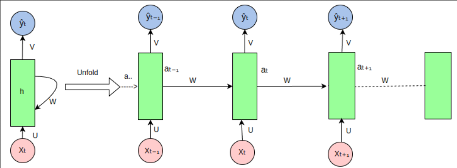
The above diagram shows the unfolding of an RNN to better understand the concept of using the output as input to the same structure.

Recurrent Neural Networks (RNNs) are defined mathematically by the way they handle sequences and update their hidden states over time. Let’s break down the key components of their mathematical representation:

Mathematical Representation of RNNs

Notation

Input Sequence: $\mathbf{x} = \{ \mathbf{x}_1, \mathbf{x}_2, \ldots, \mathbf{x}_T \}$ , where $\mathbf{x}_t$ is the input at time step $t$ and $T$ is the total length of the sequence.

Hidden State: $\mathbf{h}_t$ represents the hidden state at time step $t$ .

Output Sequence: $\mathbf{y} = \{ \mathbf{y}_1, \mathbf{y}_2, \ldots, \mathbf{y}_T \}$ , where $\mathbf{y}_t$ is the output at time step $t$ .

Hidden State Update

The core of an RNN is the recurrence relation that defines how the hidden state is updated at each time step:

$\mathbf{h}_t = f(\mathbf{W}_h \mathbf{x}_t + \mathbf{U}_h \mathbf{h}_{t-1} + \mathbf{b}_h)$

Here:

$\mathbf{W}_h$ is the weight matrix for the input at the current time step.
$\mathbf{U}_h$ is the weight matrix for the hidden state from the previous time step.
$\mathbf{b}_h$ is the bias vector.
$f$ is the activation function, commonly a non-linear function such as $\tanh$ or $\text{ReLU}$ .

Output Calculation

The output at each time step can be calculated based on the hidden state:

$\mathbf{y}_t = g(\mathbf{W}_y \mathbf{h}_t + \mathbf{b}_y)$

Here:

$\mathbf{W}_y$ is the weight matrix for the hidden state.
$\mathbf{b}_y$ is the bias vector for the output.
$g$ is the activation function for the output, often a softmax function in classification tasks.

Unfolding in Time

To better understand how RNNs work over a sequence, we can “unfold” the network in time. This unfolding reveals a network structure where each time step’s hidden state depends on the previous time step’s hidden state:

$\begin{aligned} \mathbf{h}_1 &= f(\mathbf{W}_h \mathbf{x}_1 + \mathbf{U}_h \mathbf{h}_0 + \mathbf{b}_h) \\ \mathbf{h}_2 &= f(\mathbf{W}_h \mathbf{x}_2 + \mathbf{U}_h \mathbf{h}_1 + \mathbf{b}_h) \\ &\vdots \\ \mathbf{h}_t &= f(\mathbf{W}_h \mathbf{x}_t + \mathbf{U}_h \mathbf{h}_{t-1} + \mathbf{b}_h) \\ &\vdots \\ \mathbf{h}_T &= f(\mathbf{W}_h \mathbf{x}_T + \mathbf{U}_h \mathbf{h}_{T-1} + \mathbf{b}_h) \\ \end{aligned}$

Backpropagation Through Time (BPTT)

Training RNNs involves backpropagating errors through time to update the weights. This process, known as Backpropagation Through Time (BPTT), involves unfolding the network and applying standard backpropagation to the unfolded structure.

Example Calculation

Consider a simple RNN with the following parameters:

$\mathbf{W}_h = \begin{pmatrix} 0.5 & 0.2 \\ 0.3 & 0.8 \end{pmatrix}$
$\mathbf{U}_h = \begin{pmatrix} 0.1 & 0.4 \\ 0.6 & 0.7 \end{pmatrix}$
$\mathbf{b}_h = \begin{pmatrix} 0.1 \\ 0.2 \end{pmatrix}$
Activation function $f = \tanh$

For input sequences $\mathbf{x}_1 = \begin{pmatrix} 1 \\ 0 \end{pmatrix}$ and $\mathbf{x}_2 = \begin{pmatrix} 0 \\ 1 \end{pmatrix}$ , with initial hidden state $\mathbf{h}_0 = \begin{pmatrix} 0 \\ 0 \end{pmatrix}$ :

$\begin{aligned} \mathbf{h}_1 &= \tanh(\mathbf{W}_h \mathbf{x}_1 + \mathbf{U}_h \mathbf{h}_0 + \mathbf{b}_h) \\ &= \tanh\left( \begin{pmatrix} 0.5 & 0.2 \\ 0.3 & 0.8 \end{pmatrix} \begin{pmatrix} 1 \\ 0 \end{pmatrix} + \begin{pmatrix} 0.1 & 0.4 \\ 0.6 & 0.7 \end{pmatrix} \begin{pmatrix} 0 \\ 0 \end{pmatrix} + \begin{pmatrix} 0.1 \\ 0.2 \end{pmatrix} \right) \\ &= \tanh\left( \begin{pmatrix} 0.6 \\ 0.5 \end{pmatrix} \right) \\ &= \begin{pmatrix} \tanh(0.6) \\ \tanh(0.5) \end{pmatrix} \\ &\approx \begin{pmatrix} 0.537 \\ 0.462 \end{pmatrix} \end{aligned}$

$\begin{aligned} \mathbf{h}_2 &= \tanh(\mathbf{W}_h \mathbf{x}_2 + \mathbf{U}_h \mathbf{h}_1 + \mathbf{b}_h) \\ &= \tanh\left( \begin{pmatrix} 0.5 & 0.2 \\ 0.3 & 0.8 \end{pmatrix} \begin{pmatrix} 0 \\ 1 \end{pmatrix} + \begin{pmatrix} 0.1 \cdot 0.537 + 0.4 \cdot 0.462 \\ 0.6 \cdot 0.537 + 0.7 \cdot 0.462 \end{pmatrix} + \begin{pmatrix} 0.1 \\ 0.2 \end{pmatrix} \right) \\ &= \tanh\left( \begin{pmatrix} 0.2 \\ 0.8 \end{pmatrix} + \begin{pmatrix} 0.1854 \\ 0.7552 \end{pmatrix} + \begin{pmatrix} 0.1 \\ 0.2 \end{pmatrix} \right) \\ &= \tanh\left( \begin{pmatrix} 0.5702 \\ 1.7552 \end{pmatrix} \right) \\ &\approx \begin{pmatrix} 0.515 \\ 0.942 \end{pmatrix} \end{aligned}$

Types of RNNs

Vanilla RNNs

These are the most basic types of RNNs where the output of the hidden state at time step t, is dependent on the input at time step t and output of the hidden state at time step t-1.

It has a simple architecture but is prone to vanishing and exploding gradient problems.

Long Short-Term Memory (LSTM) Networks

LSTMs are special kinds of RNNs that can form long-term dependencies. They were introduced to solve the vanishing gradient problem that is found in vanilla RNNs and contain a cell state and three types of gates: input gate, forget gate, and output gate.

They are widely used in applications such as language modeling, translation, etc.

Gated Recurrent Unit (GRU) Networks

GRUs are a simpler variant of LSTM networks. They combine the forget and input gates into a single update gate and merge the cell state and hidden state.

Bidirectional RNNs

Bidirectional RNNs process the data in both forward and backward directions. They have two hidden states, one for the forward pass and one for the backward pass. This allows them to have information from both past and future states.

Advantages and Limitations of Recurrent Neural Networks (RNNs)

Advantages

Temporal Dynamics:
- RNNs excel in capturing temporal dependencies and sequential data patterns, making them suitable for tasks like time series prediction, natural language processing (NLP), and speech recognition.
Parameter Sharing:
- Unlike traditional feedforward neural networks, RNNs share parameters across different time steps. This allows them to generalize better and handle varying sequence lengths without increasing the number of parameters.
Memory of Previous Inputs:
- Through their recurrent connections, RNNs can remember previous inputs, enabling them to maintain context and capture long-term dependencies, which is crucial for understanding sequences and contexts in data.
Flexible Input and Output Lengths:
- RNNs can process inputs of variable lengths, making them versatile for different types of sequential data. They can also generate outputs of varying lengths, which is beneficial for tasks like language translation and text generation.

Limitations

Vanishing and Exploding Gradients:
- RNNs suffer from vanishing and exploding gradient problems, which can hinder the learning process during backpropagation through time (BPTT). This issue makes it difficult for RNNs to capture long-term dependencies in sequences.
Training Complexity:
- Training RNNs can be computationally intensive and time-consuming due to their sequential nature and the need to backpropagate through each time step. This often requires specialized hardware and optimization techniques.
Difficulty in Learning Long-Term Dependencies:
- While RNNs can theoretically capture long-term dependencies, in practice, they struggle to do so effectively. Long short-term memory (LSTM) networks and gated recurrent units (GRUs) were developed to address this limitation by introducing gating mechanisms.
Limited Parallelization:
- Due to their sequential processing nature, RNNs are less efficient on parallel hardware compared to feedforward neural networks or convolutional neural networks (CNNs). This limitation can lead to slower training and inference times.
Overfitting:
- RNNs, especially when dealing with small datasets, can easily overfit due to their high expressiveness. Regularization techniques like dropout and careful tuning of hyperparameters are often required to mitigate this issue.

Conclusion

Recurrent Neural Networks (RNNs) are powerful tools for handling sequential data. They capture temporal dynamics and dependencies, making them essential for time series prediction, natural language processing, and speech recognition. RNNs excel at maintaining context and processing variable-length sequences. However, they face challenges such as the vanishing gradient problem and computational inefficiency. Advancements like LSTMs and GRUs have addressed many of these issues. This progress allows RNNs to expand their use in various fields. Understanding RNNs’ strengths and challenges is crucial for fully leveraging their potential in solving complex, time-dependent problems.